Following up on my last post about generating a Comma-Separated List of Purchase Orders for a Vendor using Excel (click here), I thought I’d show how to do the same example using Velixo Reports since Velixo Reports uses regular Excel formulas instead of DAX measure formulas. DAX measure formulas are nice, but they can be like driving a Formula 1 race car. There’s such thing as too much power 🙂
Velixo Reports is a 3rd party ISV product for Acumatica. You can learn about their recent release in this webinar video:
I’m not going to cover how to setup a Velixo Reports connection. Just know that my Velixo Connection Name is “c”. I like using “c” because my brain thinks it stands for “connection” and, more importantly, it’s only one letter which takes up the minimum amount of space when using it in an Excel formula.
I’m using the same two Generic Inquiries that we used in the last post that you can read with the link mentioned above.
Let’s use the new (fairly new) GI formula in Velixo to get the list of Vendors from Acumatica and let’s put this formula in cell A1 of a new Excel worksheet:
=GI("c","AP-Vendors",,"Vendor")
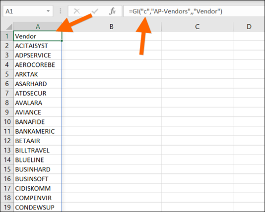
The GI Velixo Reports formula uses the new Dynamic Array Formula functionality in Excel. This is different from the old dynamic array formulas which were clunky to use and required you to remember to use Ctrl+Shift+Enter on your keyboard every time you edited them. Click here to read more about the new Dynamic Array Formulas in Excel.
Even though we put our formula in A1, notice how it automatically copied down to the cells below.
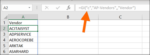
But I can’t edit the cells below. If I click on A2, you can see that the formula window shows the formula from A1, but it’s grayed out:
This list of Vendors isn’t sorted yet so let’s sort it.
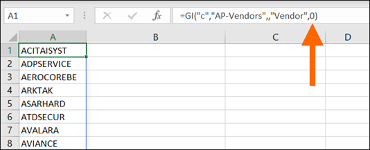
First, we don’t want it to return the Vendor column heading or else it will get sorted with the Vendors that start with “V” when we apply the sort. So let’s remove the Vendor column heading by making the last parameter in the GI function false. I like to use 0 instead of “false” because it takes up less room:
=GI("c","AP-Vendors",,"Vendor",0)
Now for the sorting part. We can wrap our formula in the SORT function which is one of the new Dynamic Array Formulas in Excel:
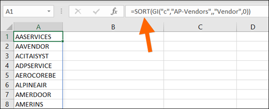
Ok, now we have a sorted list of Vendors from Acumatica.
Let’s put another formula in cell B1 that retrieves a list of Purchase Order numbers. We can do this with another GI formula:
=GI("c","PO-PurchaseOrder",,"OrderNbr",0)
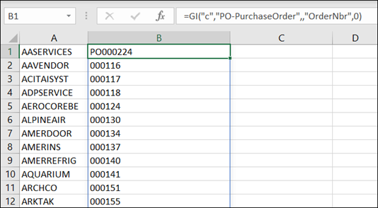
So far this just retrieves a list of all Purchase Orders in Acumatica.
Let’s make the list specific to the Vendor by adding a filter.
The filter format in the GI function uses the OData filter format. Here is a blog post that I wrote a long time ago on the official OData Blog about Acumatica OData, including some OData filter examples:
https://www.odata.org/blog/acumatica-liberates-erp-with-odata-new
And here are some additional OData filter examples:
https://www.augforums.com/forums/acumatica-odata-with-microsoft-excel-and-power-bi/applying-filters-in-odata
“Fun fact” (as my daughter likes to say) about that blog post on the OData Blog. I got invited to write that post by a guy named Gabriel Michaud who was working at Acumatica at the time. I wasn’t working at Acumatica yet, but Gabriel and I would exchange emails about reporting ideas. Gabriel came up with the idea (as far as I know) to enable OData in Acumatica which really excited me so he let me write the blog post on OData.org. Gabriel then went on years later, after leaving Acumatica, to create Velixo Reports. Pretty cool huh?
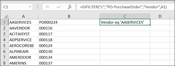
Velixo makes creating OData filters a little easier using a function called GIFILTER which returns a filter string in the format that OData expects. Let’s temporarily drop a GIFILTER function in cell C1 to see the filter format that OData expects. The OData filter string is now sitting in C1:
=GIFILTER("c","PO-PurchaseOrder","Vendor",A1)
We can embed the C1 formula in our B1 formula or even simply reference cell C1 in our B1 formula, but I’m going to copy the text from cell C1 into my B1 formula because my brain likes it better that way for some reason (just a style thing, pick what works for you):
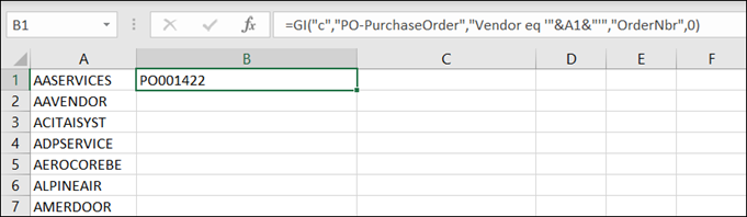
=GI("c","PO-PurchaseOrder","Vendor eq 'AASERVICES'","OrderNbr",0)
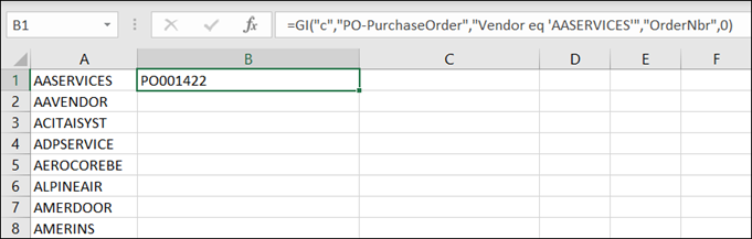
AASERVICES only has one Purchase Order so the results aren’t to exciting, but at least we know that our formula is doing something.
Before we start copying the formula down, let’s make it dynamic by replacing “AASERVICES” with a cell reference to A1:
=GI("c","PO-PurchaseOrder","Vendor eq '"&A1&"'","OrderNbr",0)
Now we can paste the formula down Column B. Let’s paste it from B1 to B6:
=GI("c","PO-PurchaseOrder","Vendor eq '"&A6&"'","OrderNbr",0)
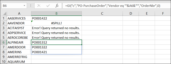
Even though we only pasted down to B6, ALPINEAIR has 3 Purchase Orders so they display as rows down to B8.
The #SPILL! value in B2 is because it wants to display multiple rows of Purchase Orders for AAVENDOR, but it can’t because we have a formula in B3. We didn’t get this behavior in Column A because we only put a formula in A1. In Column B we are putting a formula in each individual cell.
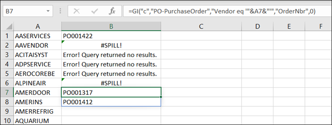
If we paste our formula down to B7, you can see that B6 becomes a #SPILL! value since it can’t display three rows of Purchase Orders, but AMERDOOR has 2 Purchase Orders so they get displayed in B7 and B8 since there is no formula yet in B8:
This is great, but these #SPILL! values are kind of annoying. Also, I want to display the Purchase Orders as a comma-separated list of values, not as rows that have the potential to return #SPILL!
Luckily for us, there is an Excel function called TEXTJOIN that can help us here.
Let’s go back up to B1 and wrap our formula in TEXTJOIN:
=TEXTJOIN(", ",1,GI("c","PO-PurchaseOrder","Vendor eq '"&A1&"'","OrderNbr",0))
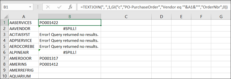
Things don’t look any different because AASERVICES only has one Purchase Order, but let’s copy our formula down to B7 and notice how those #SPILL! values get replaced with a nice comma-delimited list of Purchase Orders.
=TEXTJOIN(", ",1,GI("c","PO-PurchaseOrder","Vendor eq '"&A7&"'","OrderNbr",0))
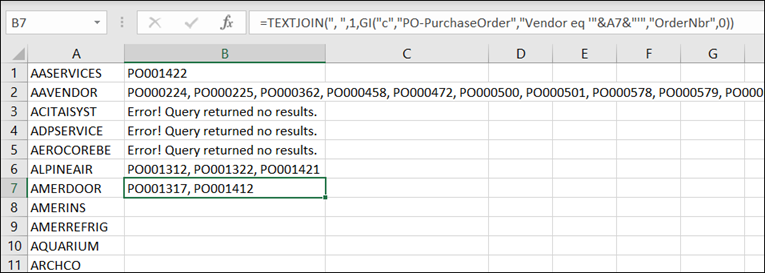
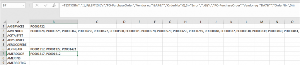
Those “Error! Query returned no results.” cells don’t look very nice so let’s go back up to B1 and modify our formula further to return an empty cell when there is an error. Then copy the B1 formula down to B7.
I wish I knew a nicer way to do this, but this is the best that I can come up with right now:
=TEXTJOIN(", ",1,IF(LEFT(GI("c","PO-PurchaseOrder","Vendor eq '"&A1&"'","OrderNbr",0),5)="Error","",GI("c","PO-PurchaseOrder","Vendor eq '"&A1&"'","OrderNbr",0)))
AAVENDOR has a lot of Purchase Orders. How about we only display the first 4 Purchase Orders, then display a “More than 4 POs” message if there are more than 4 Purchase Orders.
We can enhance our formula further like this:
=IF(COUNTA(GI("c","PO-PurchaseOrder","Vendor eq '"&A7&"'","OrderNbr",0))>4,"More than 4 Pos",TEXTJOIN(", ",1,IF(LEFT(GI("c","PO-PurchaseOrder","Vendor eq '"&A7&"'","OrderNbr",0),5)="Error","",GI("c","PO-PurchaseOrder","Vendor eq '"&A7&"'","OrderNbr",0))))

Now the results look a lot cleaner don’t they?
The formula looks pretty ugly, but the nice thing about this compared to the same example using Microsoft Excel with Power BI DAX formulas (click here) is that you don’t have to learn DAX formulas. This is just using regular Excel formulas.
And there you have it, a comma-separated list of Purchase Orders by Vendor in Acumatica!
Update February 19, 2021 from Gabriel: For large datasets, Gabriel recommends returning the data to the spreadsheet, then referencing the spreadsheet in the formulas, because it will perform better since it avoids multiple server-side queries. Also, regarding my long formula, it can be shorter in Velixo 6 which now returns error messages in something that Excel understands as an error message. This allows us to write the last formula above like this in Velixo 6:
=IF(COUNTA(GI("c","PO-PurchaseOrder","Vendor eq '"&A7&"'","OrderNbr",0))>4,"More than 4 Pos",TEXTJOIN(", ",1,IFERROR(GI("c","PO-PurchaseOrder","Vendor eq '"&A7&"'","OrderNbr",0),"")))