
Following up on a previous post about a Comma-Separated List of Shipments for a Sales Order using a Generic Inquiry and SQL View (click here), this post will be about generating a comma-separated list using Microsoft Excel.
Most people don’t realize it, but, if you are using the current Office 365 Windows Desktop version of Excel, you have access to the Power BI calculation engine as part of Excel. It’s baked in. You don’t get the fancy visualization layer that you get when using PowerBI.com, but the real “power” in “Power BI” is the calculation engine, not the visualization layer, at least that’s what I think.
So, we can use the Power BI engine inside of Excel without leaving Excel and without installing an Excel Add-In.
For this example, I’m using this Office 365 Windows Desktop version of Excel that came with my $8.25 per month subscription to Microsoft 365 Apps for business (click here).

It does need to be the Windows (not MAC) version of Desktop Excel (not Excel Online).
We’ll use two out-of-the-box Generic Inquiries for this example: Purchase Orders (PO3010PL) and Vendors (AP3030PL).
We need to enable both of these Generic Inquiries for OData using the Expose via OData checkbox on the Generic Inquiry (SM208000) screen:


Then we can go into Excel and connect to both of these Generic Inquiries using OData by going to Data -> Get Data -> From Other Sources -> From OData Feed:

I’m using my local Acumatica Instance which only has one Tenant so my OData URL looks like this:

Login with your Acumatica Username and Password. Hopefully you’re using the https protocol so you won’t get the “The password won’t be encrypted when sent.” message that I’m getting:

Check Select multiple items and check the two Generic Inquiries mentioned earlier. Then, don’t click Load, but click the down arrow next to Load and choose Load -> Load To…

Here’s where the Power BI part comes in. Rather than load the data directly into the old-fashioned Excel worksheet, we can load it into the Data Model by choosing Only Create Connection and checking Add this data to the Data Model:

If you look on the bottom, you’ll see that Excel is retrieving the data from Acumatica:

Once Excel is finished retrieving the data, you’ll see what appears to be an empty spreadsheet. Where did the data go? On the right you can see that 130 rows were loaded from AP-Vendors and 1,311 rows were loaded from PO-PurchaseOrder, but where did the data go?

If I look at the file size, it’s 821KB which is not insignificant. The empty Excel file when I started was only 9KB.

The file size got a lot bigger because the data is stored in the .xlsx Excel file. You just can’t see it in the worksheet.
To see the data, you can use this little green icon on the Data ribbon. The popup says “Go to the Power Pivot Window”. Power Pivot (formerly called PowerPivot) is the old name for Power BI.

A separate window pops up which makes it feel like you are leaving Excel, but you aren’t. Everything you see here is stored in the .xlsx file. Ah, here’s my data!

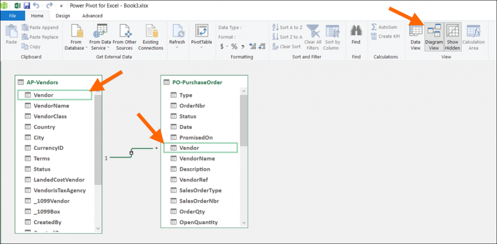
We need to create a relationship between our two data tables. To do this, go to Home -> Diagram View and drag your mouse between the Vendor field in both tables. It will draw a line between the Tables for you automatically.
Now we can close the separate window and return to our regular Excel window.
We need to create a Pivot Table so go to Insert -> PivotTable:

Rather than create a regular Pivot Table based on a range of cells (the old way), we’re going to create a Pivot Table using the Power BI functionality (the new way) by selecting Use this workbook’s Data Model:

Drag the Vendor field from the AP-Vendors table into the Rows area and drag the OrderNbr field from the PO-PurchaseOrder table into the Values area like this:

Now we have a Pivot Table which is counting the number of Purchase Orders for each Vendor.
This is nice, but I want a comma-separated list of values (Purchase Orders) for each Vendor.
To accomplish this, we need a Measure. Let’s create a Measure by right-clicking on either table and choosing Add Measure…

I’m naming my Measure POs and using the following DAX formula:
=CONCATENATEX('PO-PurchaseOrder',[OrderNbr],", ")

Drag the POs measure into the Values area and you should get a nice Pivot Table with a comma-delimited list of Purchase Orders for each Vendor:

But some of these Vendors have a lot of POs! Maybe I only want to see the list of Purchase Orders if there are 4 or less.
If there are more than 4 Purchase Orders, how about let’s display “More than 4 POs” so we don’t wind up with a really long list which forces us to scroll to the right to see them all.
Let’s right-click on the Measure and Edit Measure… so we can modify the DAX formula:

Let’s make our DAX formula a little more complicated, but not a lot more complicated.
We just want to add a check to see if the number of POs is more than 4 using this formula:
=IF(DISTINCTCOUNT('PO-PurchaseOrder'[OrderNbr])>4,"More than 4 POs",CONCATENATEX('PO-PurchaseOrder',[OrderNbr],", "))

Ah, now doesn’t that look a lot better?

There you have it, a comma-separated list of Purchase Orders for each Vendor in Acumatica using Microsoft Excel!