
By using this website, you agree to our Terms of Use (click here)

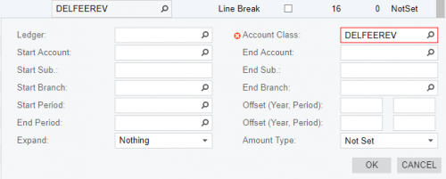
I have an income statement where the row source is delivery revenue and tied to an account class with a type of Income. We want to show this line on 1 financial statement in the expense section grouping deliveries How can I get this one line to show up as a negative with brackets (formatting is already done on the column) and I wish in red?

Thanks
Lloyd

That field, let's call it "DelRev" could be modified to be DISPLAYED as a negative, but you'll likely need to tweak any sums to reflect this. I'll cover both briefly.
Let's assume you have your cell listed as
=[DelRev]
you can change this to:
=-[DelRev]
Now your number will display as a negative value.
If your formatting is smart, you'll be fine here and can stop. If your format is not setup, you can change the text color and add symbols using .Net syntax. In the "format" field, something like:

will get you your brackets. The two backslashes are escape characters needed to allow the brackets to appear, ensure you have a single quote at the beginning and end of the line. Lastly, for display, set your font color to red.
Now we LOOK good, but your totals line (if you have one) is still going to grab [DelRev] as a positive value. I personally love using variables to get around these things. Assuming your SUM works fine for the totals, lets just add a variable to the group where [DelRev] exists that holds the value 2*DelRev. Now at your sum lets add: "=SUM(YourSumFunction)-$DelRevVar". This removes the first positive DelRev in the total and then deducts once more to include the negative DelRev.
EDIT: Image was blurred for .NET syntax, here's a text string you can paste in to the format field:
='\\[###,###.00\\]'

Thanks for jumping on this so quickly Michael.
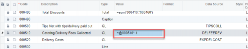
As far as I know, the only workaround for the negative thing would be to create a row that pulls the value (say it's on row @0100), set the @0100 row to be hidden by setting the Printing Control column to Hidden), then create a new row underneath it (say row @0101) with the formula =-@0100. That's really clunky, but it's the only way that I can think of.
Regarding the red, it would be a similar workaround where you would need two rows:
One row to pull in the positive values and the row is formatted in black.
Another row to pull in the negative values and the row is formatted in red.
The red solution isn't pretty either and you're probably better off just voting on this suggestion or this suggestion.
Thanks for sharing this! I never though to use a formula that references the row itself. Love it!